# A tibble: 1 × 8
     m2    df     pval  rmsea ci_lower ci_upper `90% CI`          srmsr
  <dbl> <int>    <dbl>  <dbl>    <dbl>    <dbl> <chr>             <dbl>
1 513. 325 1.26e-10 0.0141 0.0117 0.0163 [0.0117, 0.0163] 0.0319Evaluating diagnostic classification models
With Stan and measr
W. Jake Thompson, Ph.D.
Model evaluation
-
Absolute fit: How well does the model represent the observed data?
- Model-level
- Item-level
Relative fit: How do multiple models compare to each other?
Reliability: How consistent and accurate are the classifications?
Absolute model fit
Model-level absolute fit
- Limited information indices based on parameter point estimates
- M2 statistic (Liu et al., 2016)
- Posterior predictive model checks (PPMCs)
Calculating limited information indices
fit_* functions are used for calculating absolute fit indices.
Exercise 1
Open
evaluation.Rmdand run thesetupchunk.Calculate the M2 statistic for the Taylor LCDM model using
add_fit().Extract the M2 statistic. Does the model fit the data?
03:00
# A tibble: 1 × 3
     m2    df  pval
  <dbl> <int> <dbl>
1 183. 162 0.120- The null hypothesis is that our model fits the data
- p-values > .05 indicate acceptable model fit
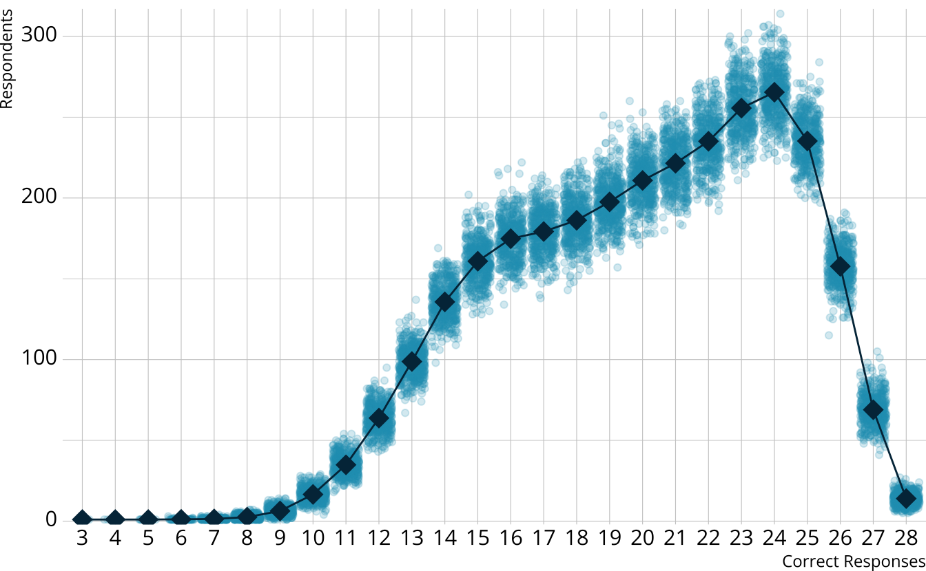
PPMC: Raw score distribution
- For each iteration, calculate the total number of respondents at each score point
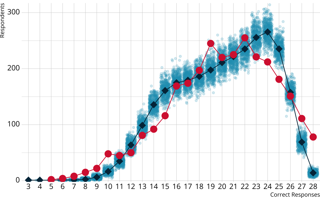
- Calculate the expected number of respondents at each score point
- Calculate the observed number of respondents at each score point

PPMC: \(\chi^2\)
- Calculate a \(\chi^2\)-like statistic comparing the number of respondents at each score point in each iteration to the expectation
- Calculate the \(\chi^2\) value comparing the observed data to the expectation
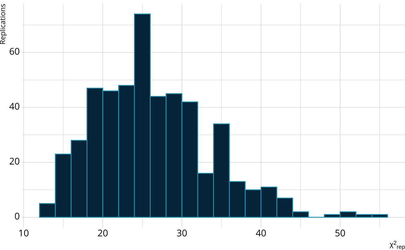
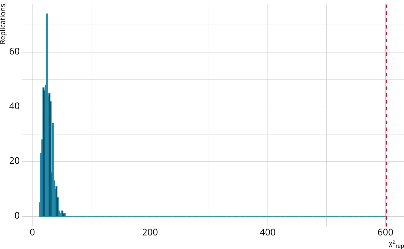
PPMC: ppp
- Calculate the proportion of iterations where the \(\chi^2\)-like statistic from replicated data set exceeds the observed data statistic
- Posterior predictive p-value (ppp)
- Very high values (e.g., >.975) or very low values (e.g., <.025) indicate our observed value is far in the tails of what the model would predict
- Poor model fit
- Ideally, we’d like ppp values close to .5
PPMCs with measr
Exercise 2
Calculate the raw score PPMC for the Taylor LCDM
Does the model fit the observed data?
04:00
taylor_lcdm <- add_fit(taylor_lcdm, method = "ppmc", item_fit = NULL)
measr_extract(taylor_lcdm, "ppmc_raw_score")
# A tibble: 1 × 5
obs_chisq ppmc_mean `2.5%` `97.5%` ppp
<dbl> <dbl> <dbl> <dbl> <dbl>
1 18.5 23.7 11.8 44.0 0.719- The ppp value is between .025 and .975
- Model fit appears to be adequate.
Item-level fit
Diagnose problems with model-level
Identify particular items that may not be performing as expected
Identify potential dimensionality issues
Item-level fit with measr
- Currently support two-measures of item-level fit using PPMCs:
- Conditional probability of each class providing a correct response (\(\pi\) matrix)
- Item pair odds ratios
Calculating item-level fit
$item_fit
$item_fit$odds_ratio
# A tibble: 378 × 7
   item_1 item_2 obs_or ppmc_mean `2.5%` `97.5%`    ppp
   <fct>  <fct>   <dbl>     <dbl>  <dbl>   <dbl>  <dbl>
 1 E1     E2       1.61      1.39   1.08    1.82 0.105
 2 E1     E3       1.42      1.49   1.22    1.79 0.642
 3 E1     E4       1.58      1.39   1.12    1.71 0.108
 4 E1     E5       1.68      1.47   1.10    1.92 0.162
 5 E1     E6       1.64      1.38   1.07    1.79 0.089
 6 E1     E7       1.99      1.71   1.39    2.11 0.0745
 7 E1     E8       1.54      1.58   1.14    2.07 0.534
 8 E1     E9       1.18      1.27   1.02    1.54 0.731
 9 E1     E10      1.82      1.59   1.28    1.93 0.104
10 E1     E11      1.61      1.63   1.30    2.00 0.536
# ℹ 368 more rowsExtracting item-level fit
# A tibble: 224 × 7
   item  class   obs_cond_pval ppmc_mean `2.5%` `97.5%`   ppp
   <fct> <chr>           <dbl>     <dbl>  <dbl>   <dbl> <dbl>
 1 E1    [0,0,0]         0.701     0.694  0.661   0.723 0.322
 2 E1    [1,0,0]         0.790     0.801  0.712   0.909 0.535
 3 E1    [0,1,0]         0.992     0.810  0.758   0.865 0
 4 E1    [0,0,1]         0.608     0.694  0.661   0.723 1
 5 E1    [1,1,0]         0.995     0.930  0.908   0.952 0
 6 E1    [1,0,1]         0.481     0.801  0.712   0.909 1
 7 E1    [0,1,1]         0.832     0.810  0.758   0.865 0.200
 8 E1    [1,1,1]         0.926     0.930  0.908   0.952 0.646
 9 E2    [0,0,0]         0.741     0.739  0.708   0.766 0.463
10 E2    [1,0,0]         0.832     0.739  0.708   0.766 0
# ℹ 214 more rows# A tibble: 378 × 7
item_1 item_2 obs_or ppmc_mean `2.5%` `97.5%` ppp
<fct> <fct> <dbl> <dbl> <dbl> <dbl> <dbl>
1 E1 E2 1.61 1.39 1.08 1.82 0.105
2 E1 E3 1.42 1.49 1.22 1.79 0.642
3 E1 E4 1.58 1.39 1.12 1.71 0.108
4 E1 E5 1.68 1.47 1.10 1.92 0.162
5 E1 E6 1.64 1.38 1.07 1.79 0.089
6 E1 E7 1.99 1.71 1.39 2.11 0.0745
7 E1 E8 1.54 1.58 1.14 2.07 0.534
8 E1 E9 1.18 1.27 1.02 1.54 0.731
9 E1 E10 1.82 1.59 1.28 1.93 0.104
10 E1 E11 1.61 1.63 1.30 2.00 0.536
# ℹ 368 more rowsFlagging item-level fit
# A tibble: 106 × 7
   item  class   obs_cond_pval ppmc_mean `2.5%` `97.5%`   ppp
   <fct> <chr>           <dbl>     <dbl>  <dbl>   <dbl> <dbl>
 1 E1    [0,1,0]         0.992     0.810  0.758   0.865 0
 2 E1    [0,0,1]         0.608     0.694  0.661   0.723 1
 3 E1    [1,1,0]         0.995     0.930  0.908   0.952 0
 4 E1    [1,0,1]         0.481     0.801  0.712   0.909 1
 5 E2    [1,0,0]         0.832     0.739  0.708   0.766 0
 6 E2    [0,1,0]         1         0.906  0.886   0.926 0
 7 E2    [0,0,1]         0.696     0.739  0.708   0.766 0.993
 8 E2    [1,1,0]         0.972     0.906  0.886   0.926 0
 9 E2    [1,0,1]         0.425     0.739  0.708   0.766 1
10 E3    [0,1,0]         0.355     0.414  0.381   0.448 1
# ℹ 96 more rows# A tibble: 80 × 7
item_1 item_2 obs_or ppmc_mean `2.5%` `97.5%` ppp
<fct> <fct> <dbl> <dbl> <dbl> <dbl> <dbl>
1 E1 E13 1.80 1.44 1.13 1.78 0.0175
2 E1 E17 2.02 1.40 1.03 1.82 0.006
3 E1 E26 1.61 1.24 1.00 1.50 0.004
4 E1 E28 1.86 1.40 1.07 1.74 0.0045
5 E2 E4 1.73 1.37 1.10 1.69 0.0145
6 E2 E14 1.64 1.23 0.994 1.52 0.003
7 E2 E15 1.92 1.46 1.08 1.90 0.02
8 E4 E5 2.81 2.09 1.58 2.75 0.0135
9 E4 E8 2.14 1.55 1.17 2.02 0.009
10 E4 E13 1.80 1.27 1.07 1.52 0
# ℹ 70 more rowsPatterns of item-level misfit
Exercise 3
Calculate PPMCs for the conditional probabilities and odds ratios for the Taylor model
What do the results tell us about the model?
05:00
# A tibble: 21 × 7
   item  class   obs_cond_pval ppmc_mean `2.5%` `97.5%`   ppp
   <fct> <chr>           <dbl>     <dbl>  <dbl>   <dbl> <dbl>
 1 1     [1,1,0]        0.972      0.880 0.831    0.923 0
 2 3     [0,0,1]        0.519      0.444 0.377    0.511 0.011
 3 5     [0,1,0]        0.417      0.333 0.262    0.407 0.015
 4 5     [0,0,1]        0.303      0.405 0.335    0.477 0.998
 5 6     [0,0,1]        0.198      0.269 0.206    0.337 0.986
 6 6     [1,0,1]        0.173      0.269 0.206    0.337 0.998
 7 7     [1,0,0]        0.0750     0.150 0.0826   0.220 0.987
 8 7     [0,1,0]        0.964      0.882 0.810    0.949 0.006
 9 9     [0,0,1]        0.794      0.724 0.662    0.788 0.018
10 13    [0,1,0]        0.325      0.452 0.383    0.520 1
# ℹ 11 more rowsRelative model fit
Model comparisons
- Doesn’t give us information whether or not a model fits the data, only compares competing models to each other
- Should be evaluated in conjunction with absolute model fit
- Implemented with the loo package
- PSIS-LOO (Vehtari, 2017)
- WAIC (Watanabe, 2010)
Relative fit with measr
Computed from 2000 by 2922 log-likelihood matrix.

         Estimate    SE
elpd_loo -42817.3 226.1
p_loo        77.1   0.8
looic     85634.5 452.1
------
MCSE of elpd_loo is 0.2.
MCSE and ESS estimates assume independent draws (r_eff=1).

All Pareto k estimates are good (k < 0.7).
See help('pareto-k-diagnostic') for details.
Comparing models
First, we need another model to compare
ecpe_dina <- measr_dcm(
  data = ecpe_data, qmatrix = ecpe_qmatrix,
  resp_id = "resp_id", item_id = "item_id",
  type = "dina",
  method = "mcmc", backend = "cmdstanr",
  iter_warmup = 1000, iter_sampling = 500,
  chains = 4, parallel_chains = 4,
  file = "fits/ecpe-dina"
)

ecpe_dina <- add_criterion(ecpe_dina, criterion = "loo")
loo_compare()
     elpd_diff se_diff
lcdm    0.0       0.0
dina -674.2 29.7 - LCDM is the preferred model
- Preferred does not imply “good”
- Remember, the LCDM showed poor absolute fit
- Difference is much larger than the standard error of the difference
- Approximate threshold: Absolute difference is greater than 2.5 × standard error of the difference (Bengio & Grandvalet, 2004)
Exercise 4
Estimate a DINA model for the Taylor data
Add PSIS-LOO and WAIC criteria to both the LCDM and DINA models for the Taylor data
-
Use
loo_compare()to compare the LCDM and DINA models- What do the findings tell us?
- Can you explain the results?
15:00
Reliability
Reliability methods
Reporting reliability depends on how results are estimated and reported
-
Reliability for:
- Profile-level classification
- Attribute-level classification
- Attribute-level probability of proficiency
Reliability with measr
$pattern_reliability
      p_a       p_c
0.7389797 0.6639670

$map_reliability
$map_reliability$accuracy
# A tibble: 3 × 8
  attribute         acc lambda_a kappa_a youden_a tetra_a  tp_a  tn_a
  <chr>           <dbl>    <dbl>   <dbl>    <dbl>   <dbl> <dbl> <dbl>
1 morphosyntactic 0.896    0.729   0.786    0.775   0.942 0.851 0.924
2 cohesive        0.852    0.675   0.703    0.699   0.892 0.877 0.822
3 lexical         0.916    0.750   0.611    0.802   0.959 0.947 0.854

$map_reliability$consistency
# A tibble: 3 × 10
  attribute       consist lambda_c kappa_c youden_c tetra_c  tp_c  tn_c gammak
  <chr>             <dbl>    <dbl>   <dbl>    <dbl>   <dbl> <dbl> <dbl>  <dbl>
1 morphosyntactic   0.834    0.557   0.685    0.646   0.853 0.779 0.867  0.852
2 cohesive          0.807    0.563   0.681    0.608   0.818 0.827 0.782  0.789
3 lexical           0.856    0.553   0.625    0.670   0.876 0.894 0.776  0.880
# ℹ 1 more variable: pc_prime <dbl>


$eap_reliability
# A tibble: 3 × 5
  attribute       rho_pf rho_bs rho_i rho_tb
  <chr>            <dbl>  <dbl> <dbl>  <dbl>
1 morphosyntactic  0.735  0.687 0.573  0.884
2 cohesive         0.729  0.574 0.506  0.785
3 lexical 0.759 0.730 0.587 0.915Profile-level classification
# A tibble: 2,922 × 9
   resp_id `[0,0,0]` `[1,0,0]` `[0,1,0]` `[0,0,1]` `[1,1,0]` `[1,0,1]` `[0,1,1]`
   <fct>       <dbl>     <dbl>     <dbl>     <dbl>     <dbl>     <dbl>     <dbl>
 1 1         7.78e-6   9.85e-5   5.14e-7  0.00131  0.0000877  0.0438     0.00207
 2 2         5.88e-6   7.44e-5   1.97e-7  0.00303  0.0000339  0.0977     0.00195
 3 3         5.64e-6   1.73e-5   1.71e-6  0.00206  0.0000687  0.00974    0.0150
 4 4         3.24e-7   4.06e-6   9.83e-8  0.000295 0.0000168  0.00988    0.00215
 5 5         1.18e-3   8.27e-3   3.55e-4  0.00127  0.0354     0.00935    0.00919
 6 6         3.01e-6   1.53e-5   9.13e-7  0.000913 0.0000633  0.00983    0.00662
 7 7         3.01e-6   1.53e-5   9.13e-7  0.000913 0.0000633  0.00983    0.00662
 8 8         3.79e-2   8.83e-5   1.35e-3  0.518    0.0000275  0.000594   0.438
 9 9         6.60e-5   1.99e-4   1.98e-5  0.00660  0.000936   0.00936    0.0480
10 10        4.14e-1   4.03e-1   3.65e-3  0.0387   0.0621     0.0181     0.00797
# ℹ 2,912 more rows
# ℹ 1 more variable: `[1,1,1]` <dbl># A tibble: 2,922 × 3
resp_id profile prob
<fct> <chr> <dbl>
1 1 [1,1,1] 0.953
2 2 [1,1,1] 0.897
3 3 [1,1,1] 0.973
4 4 [1,1,1] 0.988
5 5 [1,1,1] 0.935
6 6 [1,1,1] 0.983
7 7 [1,1,1] 0.983
8 8 [0,0,1] 0.518
9 9 [1,1,1] 0.935
10 10 [0,0,0] 0.414
# ℹ 2,912 more rows# A tibble: 1 × 2
accuracy consistency
<dbl> <dbl>
1 0.739 0.664- Estimating classification consistency and accuracy for cognitive diagnostic assessment (Cui et al., 2012)
Attribute-level classification
# A tibble: 2,922 × 4
   resp_id morphosyntactic cohesive lexical
   <fct>             <dbl>    <dbl>   <dbl>
 1 1               0.997      0.955   1.00
 2 2               0.995      0.899   1.00
 3 3               0.983      0.988   1.00
 4 4               0.998      0.990   1.00
 5 5               0.988      0.980   0.955
 6 6               0.992      0.989   1.00
 7 7               0.992      0.989   1.00
 8 8               0.00451    0.443   0.961
 9 9               0.945      0.984   0.999
10 10              0.535      0.126   0.117
# ℹ 2,912 more rows# A tibble: 2,922 × 4
resp_id morphosyntactic cohesive lexical
<fct> <int> <int> <int>
1 1 1 1 1
2 2 1 1 1
3 3 1 1 1
4 4 1 1 1
5 5 1 1 1
6 6 1 1 1
7 7 1 1 1
8 8 0 0 1
9 9 1 1 1
10 10 1 0 0
# ℹ 2,912 more rows# A tibble: 3 × 3
attribute accuracy consistency
<chr> <dbl> <dbl>
1 morphosyntactic 0.896 0.834
2 cohesive 0.852 0.807
3 lexical 0.916 0.856- Measures of agreement to assess attribute-level classification accuracy and consistency for cognitive diagnostic assessments (Johnson & Sinharay, 2018)
Attribute-level probabilities
# A tibble: 2,922 × 4
   resp_id morphosyntactic cohesive lexical
   <fct>             <dbl>    <dbl>   <dbl>
 1 1               0.997      0.955   1.00
 2 2               0.995      0.899   1.00
 3 3               0.983      0.988   1.00
 4 4               0.998      0.990   1.00
 5 5               0.988      0.980   0.955
 6 6               0.992      0.989   1.00
 7 7               0.992      0.989   1.00
 8 8               0.00451    0.443   0.961
 9 9               0.945      0.984   0.999
10 10              0.535      0.126   0.117
# ℹ 2,912 more rows# A tibble: 3 × 2
attribute informational
<chr> <dbl>
1 morphosyntactic 0.573
2 cohesive 0.506
3 lexical 0.587- The reliability of the posterior probability of skill attainment in diagnostic classification models (Johnson & Sinharay, 2020)
Exercise 5
Add reliability information to the Taylor LCDM and DINA models
Examine the attribute classification indices for both models
04:00
# A tibble: 3 × 3
  attribute   accuracy consistency
  <chr>          <dbl>       <dbl>
1 songwriting    0.969       0.941
2 production     0.910       0.837
3 vocals 0.913 0.843Evaluating diagnostic classification models
With Stan and measr