Estimating diagnostic classification models

With Stan and measr

W. Jake Thompson, Ph.D.

Example data

Data for examples

Examination for the Certificate of Proficiency in English (ECPE; Templin & Hoffman, 2013)
- 28 items measuring 3 total attributes
- 2,922 respondents
3 attributes
- Morphosyntactic rules
- Cohesive rules
- Lexical rules

ECPE data

library(measr)

ecpe_data

# A tibble: 2,922 × 29
   resp_id    E1    E2    E3    E4    E5    E6    E7    E8    E9   E10   E11
     <int> <int> <int> <int> <int> <int> <int> <int> <int> <int> <int> <int>
 1       1     1     1     1     0     1     1     1     1     1     1     1
 2       2     1     1     1     1     1     1     1     1     1     1     1
 3       3     1     1     1     1     1     1     0     1     1     1     1
 4       4     1     1     1     1     1     1     1     1     1     1     1
 5       5     1     1     1     1     1     1     1     1     1     1     1
 6       6     1     1     1     1     1     1     1     1     1     1     1
 7       7     1     1     1     1     1     1     1     1     1     1     1
 8       8     0     1     1     1     1     1     0     1     1     1     0
 9       9     1     1     1     1     1     1     1     1     1     1     1
10      10     1     1     1     1     0     0     1     1     1     1     1
# ℹ 2,912 more rows
# ℹ 17 more variables: E12 <int>, E13 <int>, E14 <int>, E15 <int>, E16 <int>,
#   E17 <int>, E18 <int>, E19 <int>, E20 <int>, E21 <int>, E22 <int>,
#   E23 <int>, E24 <int>, E25 <int>, E26 <int>, E27 <int>, E28 <int>

ECPE Q-matrix

ecpe_qmatrix

# A tibble: 28 × 4
   item_id morphosyntactic cohesive lexical
   <chr>             <int>    <int>   <int>
 1 E1                    1        1       0
 2 E2                    0        1       0
 3 E3                    1        0       1
 4 E4                    0        0       1
 5 E5                    0        0       1
 6 E6                    0        0       1
 7 E7                    1        0       1
 8 E8                    0        1       0
 9 E9                    0        0       1
10 E10                   1        0       0
# ℹ 18 more rows

Data for exercises

Multiplication data from MacReady & Dayton (1977)
Simulated Taylor Swift (and others) album assessment data

Exercise 1

Download the exercise files

usethis::use_course("measr-workshop/ncme2024-exercises")

Open estimation.Rmd
Run the setup chunk
Explore the MDM and Taylor data and Q-matrices
- How many items are in the data?
- How many respondents are in the data?
- How many attributes are measured?

03:00

MDM Data
MDM Q-Matrix
Taylor Data
Taylor Q-Matrix

mdm_data

# A tibble: 142 × 5
   respondent  mdm1  mdm2  mdm3  mdm4
   <chr>      <int> <int> <int> <int>
 1 7gray          1     1     1     1
 2 3dvje          1     1     1     1
 3 sl7fa          1     1     1     1
 4 bo4ps          1     1     1     1
 5 woxc7          1     1     1     1
 6 s9exl          1     1     1     1
 7 6cboa          1     1     1     1
 8 tckp1          1     1     1     1
 9 zfn2i          1     1     1     1
10 pre1b          1     1     1     1
# ℹ 132 more rows

4 items
142 respondents

mdm_qmatrix

# A tibble: 4 × 2
  item  multiplication
  <chr>          <int>
1 mdm1               1
2 mdm2               1
3 mdm3               1
4 mdm4               1

4 items
1 attribute
- Multiplication skills

taylor_data

# A tibble: 502 × 22
   album   `1`   `2`   `3`   `4`   `5`   `6`   `7`
   <chr> <int> <int> <int> <int> <int> <int> <int>
 1 Tayl…     0     0     0     0     0     0     0
 2 Fear…     1     0     1     0     0     0     0
 3 Fear…     1     1     0     1     0     0     0
 4 Spea…     1     0     1     0     0     0     0
 5 Spea…     1     0     0     1     1     0     0
 6 Red       1     1     0     0     1     1     1
 7 Red …     1     1     0     1     1     1     1
 8 1989      0     1     0     0     0     1     1
 9 1989…     1     1     0     1     1     1     1
10 repu…     0     1     1     0     1     0     0
# ℹ 492 more rows
# ℹ 14 more variables: `8` <int>, `9` <int>,
#   `10` <int>, `11` <int>, `12` <int>,
#   `13` <int>, `14` <int>, `15` <int>,
#   `16` <int>, `17` <int>, `18` <int>,
#   `19` <int>, `20` <int>, `21` <int>

21 items
502 albums

taylor_qmatrix

# A tibble: 21 × 3
   songwriting production vocals
         <int>      <int>  <int>
 1           1          0      0
 2           0          0      1
 3           0          1      0
 4           1          1      0
 5           1          0      1
 6           0          1      0
 7           0          1      0
 8           1          0      1
 9           0          0      1
10           1          0      1
# ℹ 11 more rows

21 items
3 attributes
- Songwriting
- Production
- Vocals

Estimation options

Existing software

Software Programs

Mplus, flexMIRT, mdltm
Limitations
- Tedious to implement, expensive, limited licenses, etc.

R Packages

CDM, GDINA, mirt, blatant
Limitations
- Limited to constrained DCMs, under-documented
- Different packages have different functionality, and don’t talk to each other

DCMs with Stan

Stan is free and open-source
Functionality is well-documented
Ecosystem of supporting packages
Existing documentation for implementing DCMs
- Case study using the DINA model
- Paper describing LCDM implmentation

Stan logo.

Stan for DCMs: Structure

Like most Stan programs, there are four main blocks:

data
parameters
transformed parameters
model

Stan for DCMs: `data`

data {
  int<lower=1> I;           // # of items
  int<lower=1> R;           // # of respondents
  int<lower=1> A;           // # of attributes
  int<lower=1> C;           // # of attribute profiles (latent classes)
  matrix[R,I] y;            // response matrix
}

Stan for DCMs: `parameters`

parameters {
  simplex[C] Vc;            // probability of class membership

  // item parameters
  real l1_0;
  real<lower=0> l1_11;
  real<lower=0> l1_12;
  real<lower=-1 * min([l1_11,l1_12])> l1_212;

  real l2_0;
  real_l2_12;
  ...
}

Item parameters in Stan

parameters {
  simplex[C] Vc;

  // item parameters
  real l1_0;
  real<lower=0> l1_11;
  real<lower=0> l1_12;
  real<lower=-1 * min([l1_11,l1_12])> l1_212;

  real l2_0;
  real_l2_12;
  ...
}

Q-matrix
Item 1
Item 2
…

# A tibble: 2 × 4
  item_id morphosyntactic cohesive lexical
  <chr>             <int>    <int>   <int>
1 E1                    1        1       0
2 E2                    0        1       0

\(\lambda_{1,0} + \lambda_{1,1(1)} + \lambda_{1,1(2)} + \lambda_{1,2(1,2)}\)

Item 1 measures attributes 1 and 2
- Intercept (l1_0)
- Two main effects (l1_11 and l1_12)
- One two-way interaction (l1_212)

\(\lambda_{2,0} + \lambda_{2,1(2)}\)

Item 2 measures only attribute 2
- Intercept (l2_0)
- One main effect (l2_12)

Repeat for all remaining items.

Stan for DCMs: `transformed parameters`

transformed parameters {
  matrix[I,C] PImat;

  PImat[1,1] = inv_logit(l1_0);
  PImat[1,2] = inv_logit(l1_0 + l1_1);
  PImat[1,3] = inv_logit(l1_0 + l1_2);
  PImat[1,4] = inv_logit(l1_0);
  PImat[1,5] = inv_logit(l1_0 + l1_11 + l1_12 + l1_212);
  PImat[1,6] = inv_logit(l1_0 + l1_1);
  PImat[1,7] = inv_logit(l1_0 + l1_2);
  PImat[1,8] = inv_logit(l1_0 + l1_11 + l1_12 + l1_212);
  ...
}

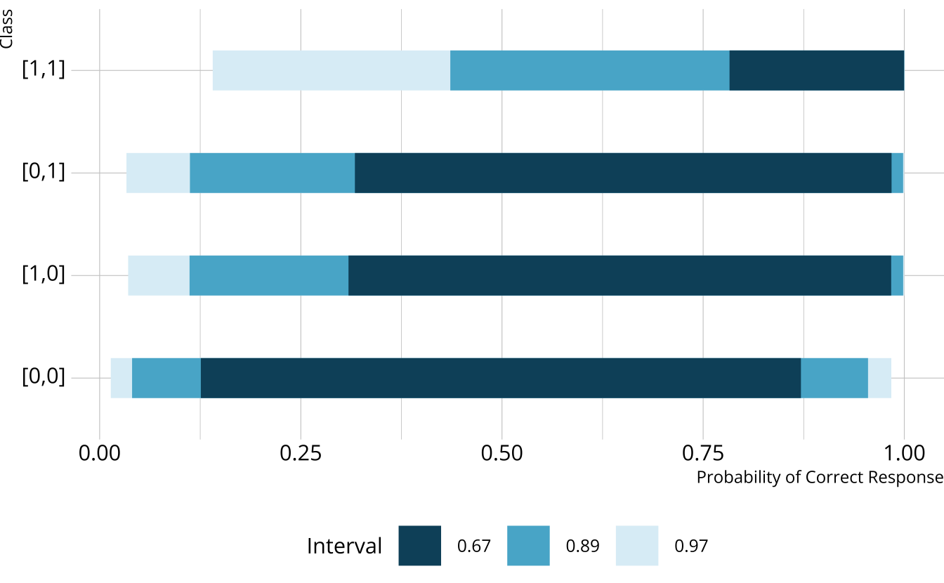
DCM classes

When using binary attributes, there are 2^A possible profiles

create_profiles(3)

# A tibble: 8 × 3
   att1  att2  att3
  <int> <int> <int>
1     0     0     0
2     1     0     0
3     0     1     0
4     0     0     1
5     1     1     0
6     1     0     1
7     0     1     1
8     1     1     1

Mapping classes to `PImat`

transformed parameters {
  matrix[I,C] PImat;

  PImat[1,1] = inv_logit(l1_0);
  PImat[1,2] = inv_logit(l1_0 + l1_1);
  PImat[1,3] = inv_logit(l1_0 + l1_2);
  PImat[1,4] = inv_logit(l1_0);
  PImat[1,5] = inv_logit(l1_0 + l1_11 + l1_12 + l1_212);
  PImat[1,6] = inv_logit(l1_0 + l1_1);
  PImat[1,7] = inv_logit(l1_0 + l1_2);
  PImat[1,8] = inv_logit(l1_0 + l1_11 + l1_12 + l1_212);
  ...
}

create_profiles(3)

# A tibble: 8 × 3
   att1  att2  att3
  <int> <int> <int>
1     0     0     0
2     1     0     0
3     0     1     0
4     0     0     1
5     1     1     0
6     1     0     1
7     0     1     1
8     1     1     1

Stan for DCMs: `model`

\(P(X_r=x_r) = \sum_{c=1}^C\nu_c \prod_{i=1}^I\pi_{ic}^{x_{ir}}(1-\pi_{ic})^{1 - x_{ir}}\)

model {
  for (r in 1:R) {
    real ps[C];
    for (c in 1:C) {
      real log_items[I];
      for (i in 1:I) {
        log_items[i] = y[r,i] * log(PImat[i,c]) + (1 - y[r,i]) * log(1 - pi[i,c]);
      }
      ps[c] = log(Vc[c]) + sum(log_items);
    }
    target += log_sum_exp(ps);
  }
}

Exercise 2

Complete the parameters and transformed parameters blocks for the MDM data.

05:00

parameters {
  simplex[C] Vc;

  // item parameters
  real l1_0;
  real<lower=0> l1_11;
  real l2_0;
  real<lower=0> l2_11;
  real l3_0;
  real<lower=0> l3_11;
  real l4_0;
  real<lower=0> l4_11;
}
transformed parameters {
  matrix[I,C] PImat;

  PImat[1,1] = inv_logit(l1_0);
  PImat[1,2] = inv_logit(l1_0 + l1_11);
  PImat[2,1] = inv_logit(l2_0);
  PImat[2,2] = inv_logit(l2_0 + l2_11);
  PImat[3,1] = inv_logit(l3_0);
  PImat[3,2] = inv_logit(l3_0 + l3_11);
  PImat[4,1] = inv_logit(l4_0);
  PImat[4,2] = inv_logit(l4_0 + l4_11);
}

Limitations of Stan for DCMs

Very tedious—prone to typos
Complexity increases with the number of attributes and item structure
parameters and transformed parameters blocks have to be customized to each particular Q-matrix

Benefits of Stan for DCMs

Powerful and flexible
Access to other packages in the Stan ecosystem
- loo
- tidybayes
- posterior
Just need to automate the creation of the Stan scripts…

What is measr?

R package that automates the creation of Stan scripts for DCMs
Wraps rstan or cmdstanr to estimate the models
Provides additional functions to automate the evaluation of DCMs
- Model fit
- Classification accuracy and consistency

`measr_dcm()`

Estimate a DCM with Stan

ecpe <- measr_dcm(
  data = ecpe_data, qmatrix = ecpe_qmatrix,
  resp_id = "resp_id", item_id = "item_id",
  type = "lcdm",
  method = "mcmc", backend = "cmdstanr",
  iter_warmup = 1000, iter_sampling = 500,
  chains = 4, parallel_chains = 4,
  file = "fits/ecpe-lcdm"
)

1: Specify your data, Q-matrix, and ID columns
2: Choose the DCM to estimate (e.g., LCDM, DINA, etc.)
3: Choose the estimation engine
4: Pass additional arguments to rstan or cmdstanr
5: Save the model to save time in the future

`measr_dcm()` options

type: Declare the type of DCM to estimate. Currently support LCDM, DINA, DINO, and C-RUM
method: How to estimate the model. To sample, use “mcmc”. To use Stan’s optimizer, use “optim”
backend: Which engine to use, either “rstan” or “cmdstanr”
...: Additional arguments that are passed to, depending on the method and backend:

Exercise 3

Estimate an LCDM on the Taylor data. Your model should have:

2 chains
1000 warmup and 500 sampling iterations
Use whichever backend you prefer

15:00

taylor_lcdm <- measr_dcm(
  data = taylor_data, qmatrix = taylor_qmatrix,
  resp_id = "album",
  type = "lcdm",
  method = "mcmc", backend = "rstan",
  warmup = 1000, iter = 1500,
  chains = 2, cores = 2,
  file = "fits/taylor-lcdm"
)

Extracting item parameters

measr_extract() can be used to pull out components of an estimated model.

measr_extract(ecpe, "item_param")

# A tibble: 74 × 5
   item_id class       attributes                coef         estimate
   <fct>   <chr>       <chr>                     <glue>     <rvar[1d]>
 1 E1      intercept   <NA>                      l1_0     0.82 ± 0.075
 2 E1      maineffect  morphosyntactic           l1_11    0.61 ± 0.368
 3 E1      maineffect  cohesive                  l1_12    0.64 ± 0.212
 4 E1      interaction morphosyntactic__cohesive l1_212   0.53 ± 0.481
 5 E2      intercept   <NA>                      l2_0     1.04 ± 0.077
 6 E2      maineffect  cohesive                  l2_12    1.23 ± 0.152
 7 E3      intercept   <NA>                      l3_0    -0.35 ± 0.072
 8 E3      maineffect  morphosyntactic           l3_11    0.74 ± 0.389
 9 E3      maineffect  lexical                   l3_13    0.36 ± 0.116
10 E3      interaction morphosyntactic__lexical  l3_213   0.53 ± 0.406
# ℹ 64 more rows

Extracting structural parameters

measr_extract(ecpe, "strc_param")

# A tibble: 8 × 2
  class           estimate
  <chr>         <rvar[1d]>
1 [0,0,0]  0.2983 ± 0.0168
2 [1,0,0]  0.0118 ± 0.0066
3 [0,1,0]  0.0162 ± 0.0106
4 [0,0,1]  0.1278 ± 0.0198
5 [1,1,0]  0.0095 ± 0.0058
6 [1,0,1]  0.0184 ± 0.0102
7 [0,1,1]  0.1726 ± 0.0202
8 [1,1,1]  0.3454 ± 0.0177

Extracting respondent probabilities

ecpe <- add_respondent_estimates(ecpe)
measr_extract(ecpe, "attribute_prob")

# A tibble: 2,922 × 4
   resp_id morphosyntactic cohesive lexical
   <fct>             <dbl>    <dbl>   <dbl>
 1 1               0.997      0.955   1.00 
 2 2               0.995      0.899   1.00 
 3 3               0.983      0.988   1.00 
 4 4               0.998      0.990   1.00 
 5 5               0.988      0.980   0.955
 6 6               0.992      0.989   1.00 
 7 7               0.992      0.989   1.00 
 8 8               0.00451    0.443   0.961
 9 9               0.945      0.984   0.999
10 10              0.535      0.126   0.117
# ℹ 2,912 more rows

Exercise 4

What proportion of respondents have mastered both songwriting and vocals in the Taylor data?

What is the probability that folklore has mastered vocals?

02:00

Structural parameters
Respondent probabilities

measr_extract(taylor_lcdm,
              "strc_param")

# A tibble: 8 × 2
  class         estimate
  <chr>       <rvar[1d]>
1 [0,0,0]  0.158 ± 0.021
2 [1,0,0]  0.119 ± 0.019
3 [0,1,0]  0.081 ± 0.018
4 [0,0,1]  0.115 ± 0.019
5 [1,1,0]  0.122 ± 0.019
6 [1,0,1]  0.131 ± 0.020
7 [0,1,1]  0.138 ± 0.020
8 [1,1,1]  0.136 ± 0.022

measr_extract(taylor_lcdm,
              "strc_param") |> 
  slice(c(6, 8)) |> 
  summarize(estimate = rvar_sum(estimate))

# A tibble: 1 × 1
       estimate
     <rvar[1d]>
1  0.27 ± 0.027

taylor_lcdm <- add_respondent_estimates(taylor_lcdm)
measr_extract(taylor_lcdm, "attribute_prob") |> 
  filter(album == "folklore")

# A tibble: 1 × 4
  album    songwriting production vocals
  <fct>          <dbl>      <dbl>  <dbl>
1 folklore        1.00      0.995  0.913

Working with Stan objects

Extract Stan code with:

ecpe$stancode

Extract the Stan object:

ecpe$model

Priors

Default priors

default_dcm_priors(type = "lcdm")

# A tibble: 4 × 3
  class       coef  prior_def                  
  <chr>       <chr> <chr>                      
1 intercept   <NA>  normal(0, 2)               
2 maineffect  <NA>  lognormal(0, 1)            
3 interaction <NA>  normal(0, 2)               
4 structural  Vc    dirichlet(rep_vector(1, C))

Weakly informative priors

The distribution of expected probabilities of providing a correct response for each class, based on the default priors.

Creating custom priors

prior(normal(0, 10), class = "maineffect")

# A tibble: 1 × 3
  class      coef  prior_def    
  <chr>      <chr> <chr>        
1 maineffect <NA>  normal(0, 10)

prior(normal(0, 1), class = "intercept", coef = "l3_0")

# A tibble: 1 × 3
  class     coef  prior_def   
  <chr>     <chr> <chr>       
1 intercept l3_0  normal(0, 1)

my_prior <- prior(normal(-1, 1), class = "intercept")
new_ecpe <- measr_dcm(
  data = ecpe_data, qmatrix = ecpe_qmatrix,
  resp_id = "resp_id", item_id = "item_id",
  type = "lcdm",
  prior = my_prior,
  method = "optim", backend = "cmdstanr",
  file = "fits/ecpe-new-prior"
)

new_ecpe <- measr_dcm(
  data = ecpe_data, qmatrix = ecpe_qmatrix,
  resp_id = "resp_id", item_id = "item_id",
  type = "lcdm",
  prior = prior(normal(-1, 1), class = "intercept"),
  method = "optim", backend = "cmdstanr",
  file = "fits/ecpe-new-prior"
)

Extract priors

measr_extract(ecpe, "prior")

# A tibble: 4 × 3
  class       coef  prior_def                  
  <chr>       <chr> <chr>                      
1 intercept   <NA>  normal(0, 2)               
2 maineffect  <NA>  lognormal(0, 1)            
3 interaction <NA>  normal(0, 2)               
4 structural  Vc    dirichlet(rep_vector(1, C))

measr_extract(new_ecpe, "prior")

# A tibble: 4 × 3
  class       coef  prior_def                  
  <chr>       <chr> <chr>                      
1 intercept   <NA>  normal(-1, 1)              
2 maineffect  <NA>  lognormal(0, 1)            
3 interaction <NA>  normal(0, 2)               
4 structural  Vc    dirichlet(rep_vector(1, C))

Exercise 5

Estimate a new LCDM model for the Taylor data with the following priors:

Intercepts: normal(-1, 2)
- Except item 3, which should use a normal(0, 1) prior
Main effects: lognormal(0, 1)

Use backend = "optim" for a speedier estimation

Extract the prior to see that the specifications were applied

05:00

new_taylor <- measr_dcm(
  data = taylor_data, qmatrix = taylor_qmatrix,
  resp_id = "album",
  type = "lcdm",
  prior = c(prior(normal(-1, 2), class = "intercept"),
            prior(normal(0, 1), class = "intercept", coef = "l3_0")),
  method = "optim", backend = "rstan",
  file = "fits/taylor-new-prior"
)

measr_extract(new_taylor, "prior")

# A tibble: 5 × 3
  class       coef  prior_def                  
  <chr>       <chr> <chr>                      
1 intercept   <NA>  normal(-1, 2)              
2 intercept   l3_0  normal(0, 1)               
3 maineffect  <NA>  lognormal(0, 1)            
4 interaction <NA>  normal(0, 2)               
5 structural  Vc    dirichlet(rep_vector(1, C))

Estimating diagnostic classification models

With Stan and measr

https://ncme2024.measr.info

Estimating diagnostic classification models

Example data

Data for examples

ECPE data

ECPE Q-matrix

Data for exercises

Exercise 1

Estimation options

Existing software

DCMs with Stan

Stan for DCMs: Structure

Stan for DCMs: data

Stan for DCMs: parameters

Item parameters in Stan

Stan for DCMs: transformed parameters

DCM classes

Mapping classes to PImat

Stan for DCMs: model

Exercise 2

Limitations of Stan for DCMs

Benefits of Stan for DCMs

What is measr?

measr_dcm()

measr_dcm() options

Exercise 3

Extracting item parameters

Extracting structural parameters

Extracting respondent probabilities

Exercise 4

Working with Stan objects

Priors

Default priors

Weakly informative priors

Creating custom priors

Specifying custom priors

Extract priors

Exercise 5

Stan for DCMs: `data`

Stan for DCMs: `parameters`

Stan for DCMs: `transformed parameters`

Mapping classes to `PImat`

Stan for DCMs: `model`

`measr_dcm()`

`measr_dcm()` options