Terminology
Respondents (r): The individuals from whom behavioral data are collected
- For today, this is dichotomous assessment item responses
- Not limited to only item responses in practice
Items (i): Assessment questions used to classify/diagnose respondents
Attributes (a): Unobserved latent categorical characteristics underlying the behaviors (i.e., diagnostic status)
Diagnostic Assessment: The method used to elicit behavioral data
Attribute profiles
[0, 0, 0]
[1, 0, 0]
[0, 1, 0]
[0, 0, 1]
[1, 1, 0]
[1, 0, 1]
[0, 1, 1]
[1, 1, 1]
DCMs as latent class models
\[
\color{#D55E00}{P(X_r=x_r)} = \sum_{c=1}^C\color{#009E73}{\nu_c} \prod_{i=1}^I\color{#56B4E9}{\pi_{ic}^{x_{ir}}(1-\pi_{ic})^{1 - x_{ir}}}
\]
Observed data: Probability of observing examinee r's item reponses
Structural component: Proportion of examinees in each class
Measurement component: Product of item response probabilities
Structural models
\[
\color{#D55E00}{P(X_r=x_r)} = \sum_{c=1}^C\color{#009E73}{\nu_c} \prod_{i=1}^I\color{#56B4E9}{\pi_{ic}^{x_{ir}}(1-\pi_{ic})^{1 - x_{ir}}}
\]
Structural component: Proportion of examinees in each class
- Prevalence of each class in the population
- Typically unconstrained
Measurement models
\[
\color{#D55E00}{P(X_r=x_r)} = \sum_{c=1}^C\color{#009E73}{\nu_c} \prod_{i=1}^I\color{#56B4E9}{\pi_{ic}^{x_{ir}}(1-\pi_{ic})^{1 - x_{ir}}}
\]
Measurement component: Product of item response probabilities
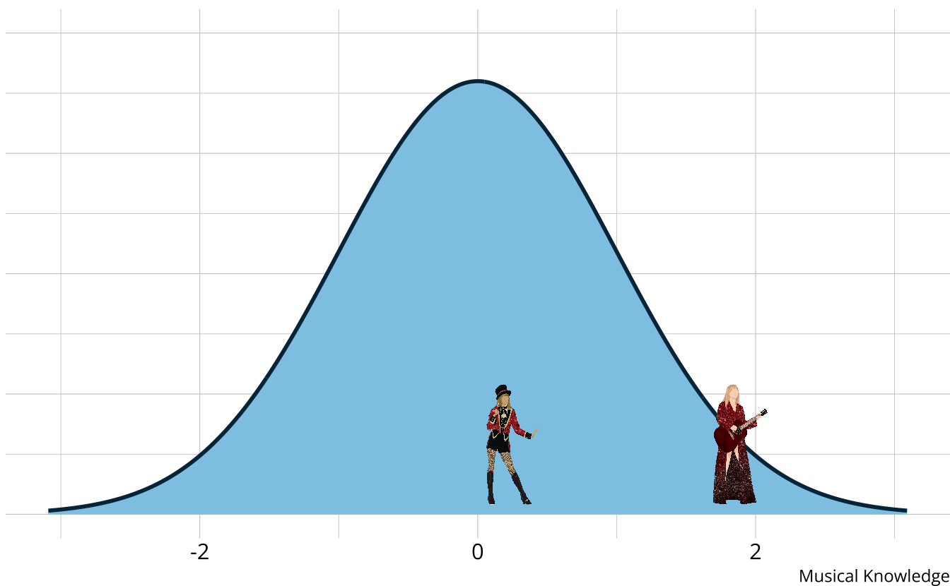
- Traditional psychometrics: Item response theory, classical test theory
- A single, unidimensional construct
- Student results estimated on a continuum
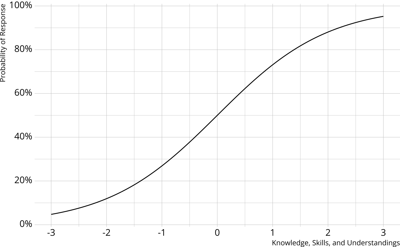
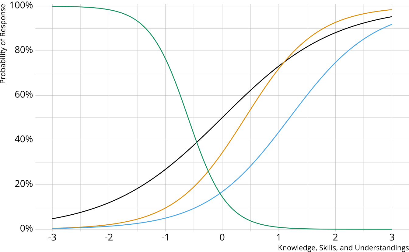
- Performance on individual items determined by an “item characteristic curve”
- DCMs: Many different options
Diagnostic assessment items
DCM measurement models
Items can measure one or both attributes
Different DCMs define πic in different ways
- Each DCM makes different assumptions about how attributes proficiencies combine/interact to produce an item response
Item characteristic bar charts
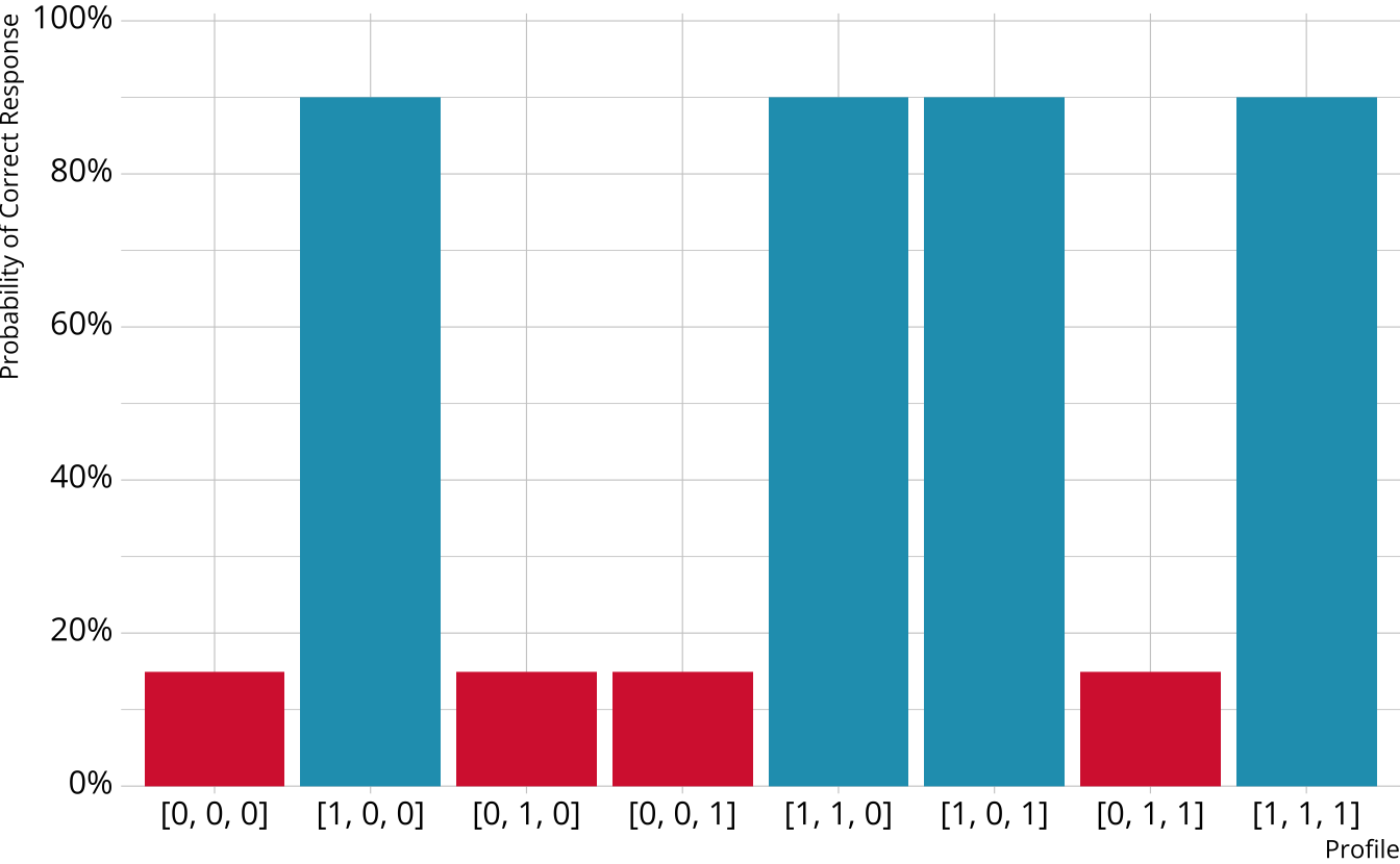
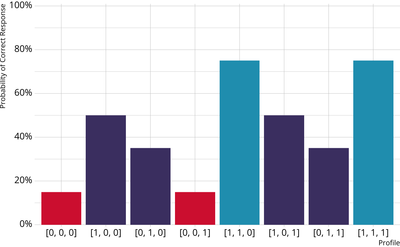
Single-attribute DCM item
Item measures just attribute 1
Respondents who are proficient on attribute 1 have high probability of correct response, regardless of other attributes
Multi-attribute items
When items measure multiple attributes, what level of mastery is needed in order to provide a correct response?
Many different types of DCMs that define this probability differently
- Compensatory (e.g., DINO)
- Noncompensatory (e.g., DINA)
- Partially compensatory (e.g., C-RUM)
General diagnostic models (e.g., LCDM)
Each DCM makes different assumptions about how attributes proficiencies combine/interact to produce an item response
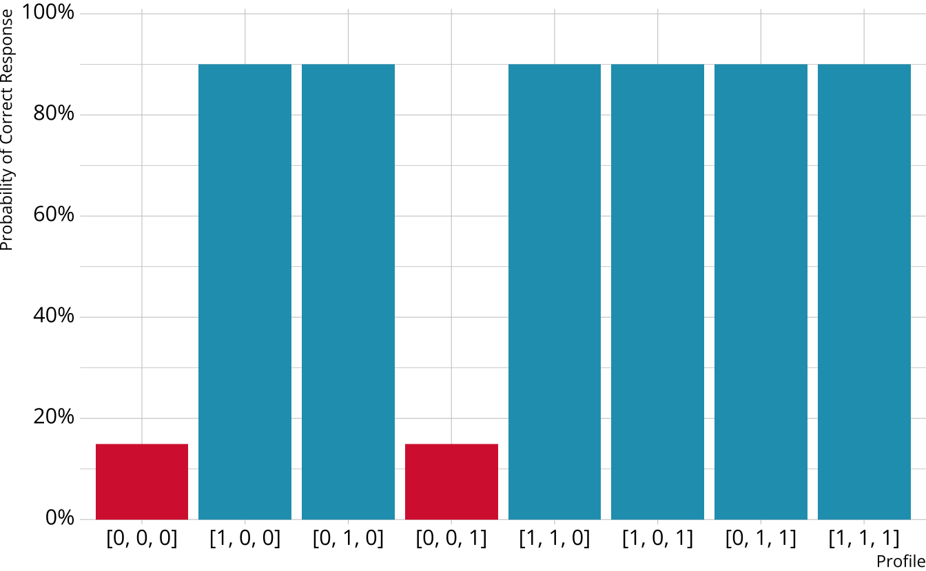
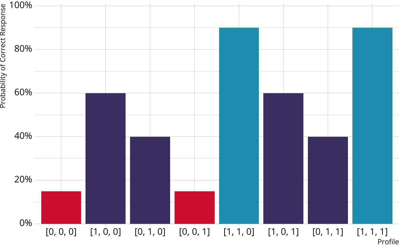
Compensatory DCMs
Item measures attributes 1 and 2
Must be proficient in at least 1 attribute measured by the item to provide a correct response
Deterministic inputs, noisy “or” gate (DINO; Templin & Henson, 2006)
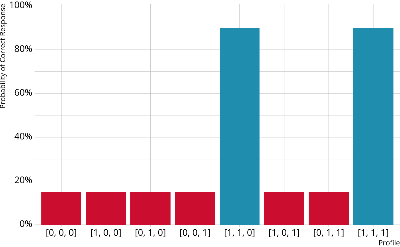
Non-compensatory DCMs
Item measures attributes 1 and 2
Must be proficient in all attributes measured by the item to provide a correct response
Deterministic inputs, noisy “and” gate (DINA; de la Torre & Douglas, 2004)
Partially Compensatory DCMs
Separate increases for each acquired attribute
Compensatory reparameterized unified model (C-RUM; Hartz, 2002)
Which DCM to use?
DINO, DINA, and C-RUM are just 3 of the MANY models that are available
Each model comes with its own set of restrictions, and we typically have to specify a single model that is used for all items (software constraint)
General form diagnostic models
- Flexible; can subsume other more restrictive models
- Again, several possibilities (e.g., G-DINA, GDM, LCDM)
General DCMs
Different response probabilities for each class (partially compensatory)
Log-linear cognitive diagnostic model (LCDM; Henson et al., 2009)
This will be our focus
Simple structure LCDM
Item measures only 1 attribute
\[
\text{logit}(X_i = 1) = \color{#D7263D}{\lambda_{i,0}} + \color{#219EBC}{\lambda_{i,1(1)}}\color{#009E73}{\alpha}
\]
λi,0: Log-odds when not proficient
λi,1(1): Increase in log-odds when proficient
α: Attribute proficiency status (either 0 or 1)
Subscript notation
- i = The item to which the parameter belongs
- e = The level of the effect
- 0 = intercept
- 1 = main effect
- 2 = two-way interaction
- 3 = three-way interaction
- Etc.
- (α1,…) = The attributes to which the effect applies
- The same number of attributes as listed in subscript 2
Complex structure LCDM
Item measures multiple attributes
\[
\text{logit}(X_i = 1) = \color{#D7263D}{\lambda_{i,0}} + \color{#4B3F72}{\lambda_{i,1(1)}\alpha_1} + \color{#9589BE}{\lambda_{i,1(2)}\alpha_2} +
\color{#219EBC}{\lambda_{i,2(1,2)}\alpha_1\alpha_2}
\]
Log-odds when proficient in neither attribute
Increase in log-odds when proficient in attribute 1
Increase in log-odds when proficient in attribute 2
Change in log-odds when proficient in both attributes
The LCDM as a general DCM
So called “general” DCM because the LCDM subsumes other DCMs
Constraints on item parameters make LCDM equivalent to other DCMs (e.g., DINA and DINO)
- DINA
- Only the intercept and highest-order interaction are non-0
- DINO
- All main effects are equal
- All two-way interactions are -1 \(\times\) main effect
- All three-way interactions are -1 \(\times\) two-way interaction (i.e., equal to main effects)
- Etc.
- C-RUM
- Only the intercept and main effects are non-0 (i.e., interactions are not estimated)
- Interactive Shiny app: https://atlas-aai.shinyapps.io/dcm-probs/
From model parameters to respondents
Respondent estimates come from combining the estimated model parameters with the response data
For DCMs, a similar process to that for IRT
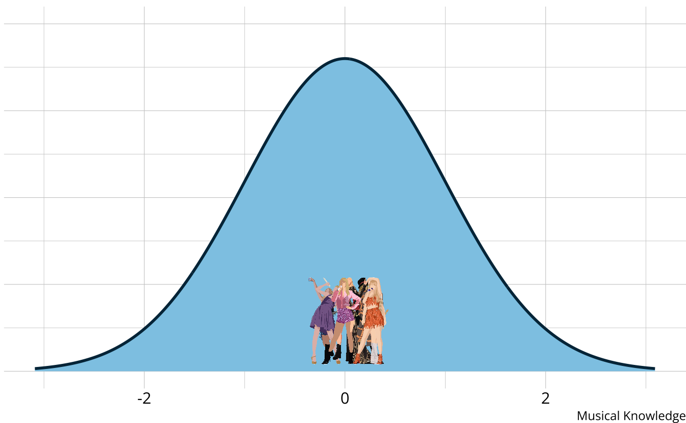
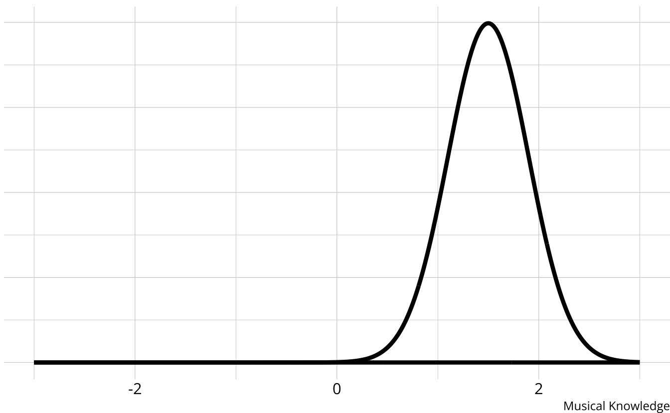
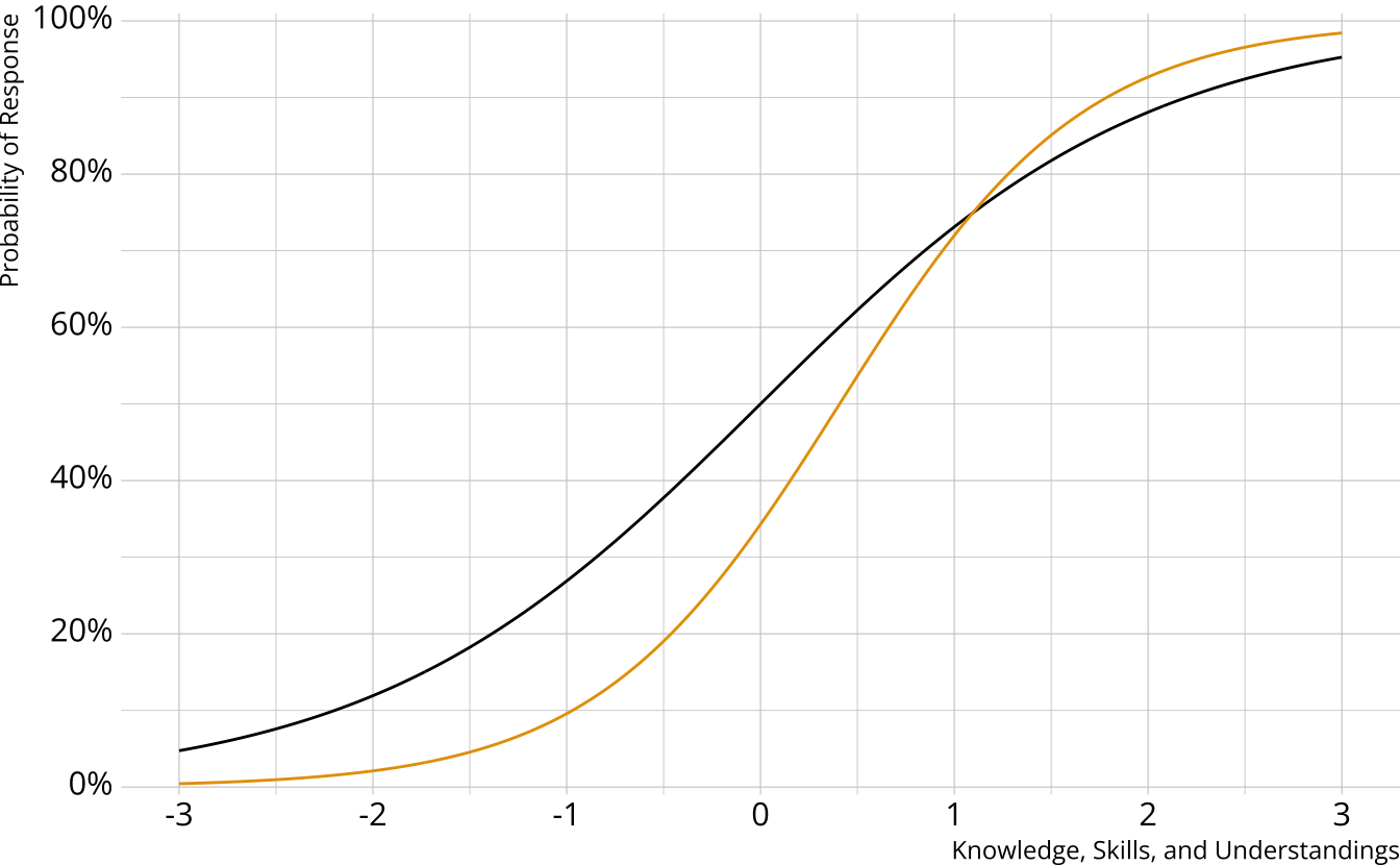
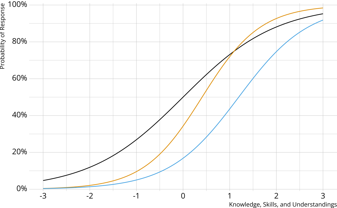
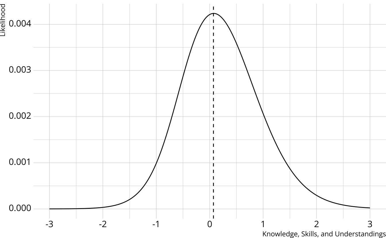
IRT respondent estimate
Multiply the ICCs together
- Multiply the response probabilities together for each value of the trait
Student estimate is the peak of the curve
Spread of the curve represents uncertainty in estimate
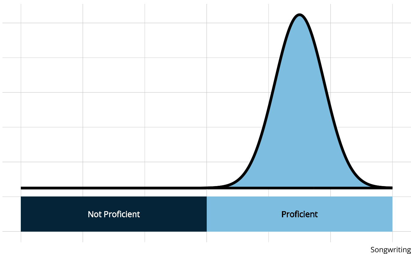
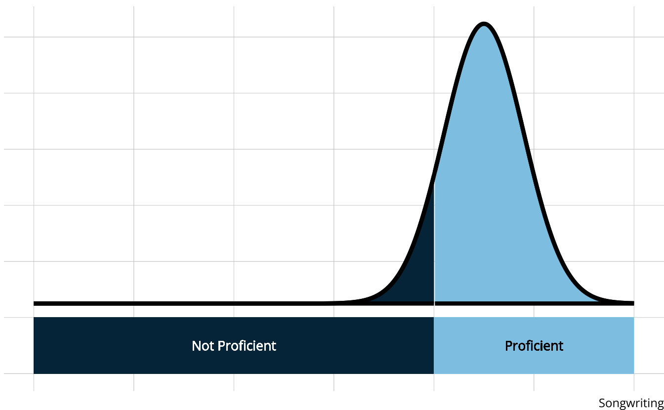
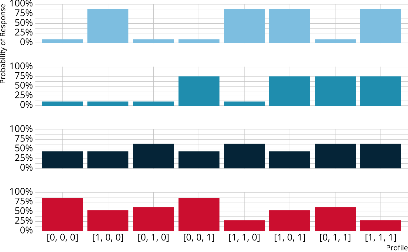
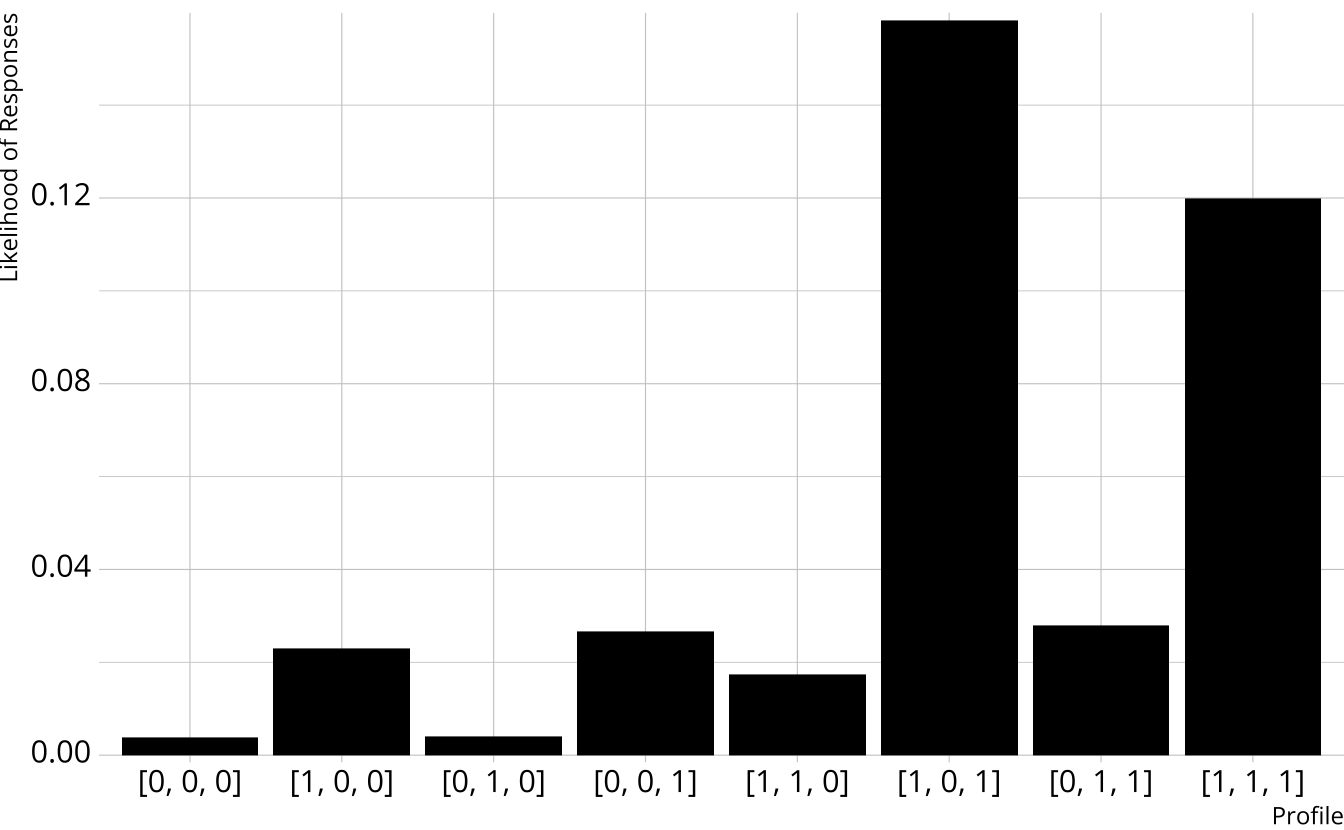
DCM respondent estimate
- Multiply the response probabilities together for each class
- Multiply the item response likelihoods by structural parameters
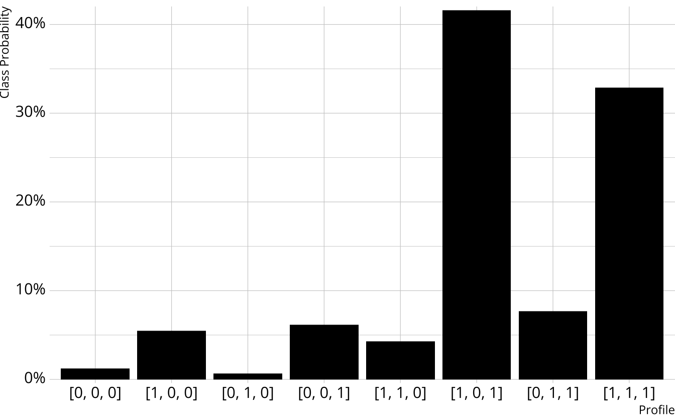
- Class probabilities are the class likelihoods divided by the total likelihood
From class to attribute probabilities
- For each attribute, sum the class probabilities where that attribute is present
| 0 |
0 |
0 |
0.012 |
| 1 |
0 |
0 |
0.055 |
| 0 |
1 |
0 |
0.007 |
| 0 |
0 |
1 |
0.062 |
| 1 |
1 |
0 |
0.043 |
| 1 |
0 |
1 |
0.416 |
| 0 |
1 |
1 |
0.077 |
| 1 |
1 |
1 |
0.329 |
|
|
|
0.842 |
| 0 |
0 |
0 |
0.012 |
| 1 |
0 |
0 |
0.055 |
| 0 |
1 |
0 |
0.007 |
| 0 |
0 |
1 |
0.062 |
| 1 |
1 |
0 |
0.043 |
| 1 |
0 |
1 |
0.416 |
| 0 |
1 |
1 |
0.077 |
| 1 |
1 |
1 |
0.329 |
|
|
|
0.455 |
| 0 |
0 |
0 |
0.012 |
| 1 |
0 |
0 |
0.055 |
| 0 |
1 |
0 |
0.007 |
| 0 |
0 |
1 |
0.062 |
| 1 |
1 |
0 |
0.043 |
| 1 |
0 |
1 |
0.416 |
| 0 |
1 |
1 |
0.077 |
| 1 |
1 |
1 |
0.329 |
|
|
|
0.884 |